We, at Les Fées Spéciales, love the Blender Grease Pencil. Not only it allows you to draw and animate in 2D, but it also allows you to do it in 3D directly in the Blender scene.
Why not use it to sketch 3D surfaces, then ? With a few strokes, we would be able to populate a 3D animation with FX elements, for example. In this scope, we implemented an algorithm to triangulate grease pencil strokes.
This article exists in French / Cet article existe en français.
An example of 3D grease pencil stroke in Blender
This system raises the question of triangulation, because the drawn strokes might not be planar, and the camera might not be set front to the drawing. Actually, each grease pencil stroke comes with a triangulation, accessible from the python API.
However, the proposed triangulation has poor mesh qualities : many triangles are degenerated, and discontinuities often appears, when the stroke boundary is not planar. One of the main reason is that the mesh contains no other vertices than the boundary.
A possible way to improve this triangulation would be to subdivide each triangle by adding its barycenter to the set of vertices. With a few Blender operators, we can then beautify the faces, and transform triangles to quads when possible. Still, there is no guarantee in the quality of the resulting mesh.
In this post, we present the method we implemented to solve this issue. This method is not new, inspired by the scientific literature on this topic, which is cited within the text. Notably, a similar method was used for triangulation of curve networks [Stanko et al. 16].
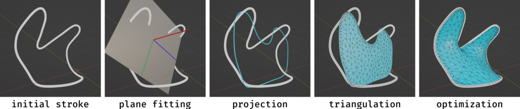
Overview of the triangulation method
Local frame
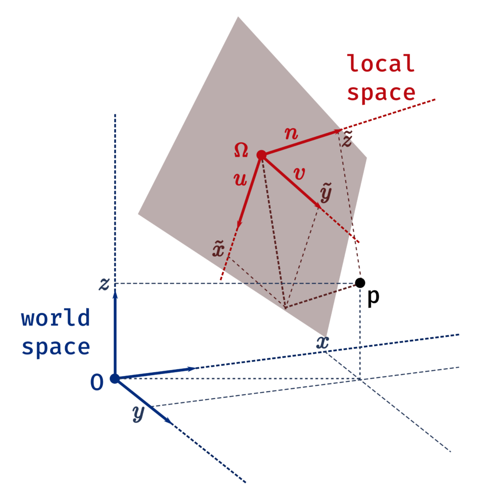
First, we need to compute a local frame in which we can perform our 2D triangulation. We find the normal of the best fitting plane by computing the eigenvectors of the covariance matrix of the points. If you are not familiar with these, no worries, the numpy library will compute them for us anyways. The idea is that the eigenvectors of the covariance matrix form a set of vectors that are orthogonal in 3D, and point to directions of least to most variance of points. We choose the direction in which the points vary the least to be the plane normal.
# Barycenter and centered coordinates
bar = barycenter(verts)
x = np.asarray([v - bar for v in verts])
# Covariance matrix and eigenvalues
M = np.cov(x.T)
eigenvalues,eigenvectors = np.linalg.eig(M)
# Local frame
# u : direction of most variance of the coordinates
# n : direction of least variance of the coordinates
# => normal of the fitting plane
# v : vector orthogonal to both u and n
u = Vector(eigenvectors[:,eigenvalues.argmax()])
n = Vector(eigenvectors[:,eigenvalues.argmin()])
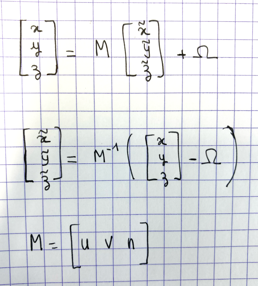
v = n.cross(u)We now have an orthonormal frame, meaning 3 unit vectors (u,v,n) which are orthogonal, and a local origin Ω which is computed as the barycenter of all points in the stroke. We can switch any point coordinate from the global (world) space to the local frame space using the basis change matrix M= [u v n], with the following formula.
2D Triangulation
We can now compute 2D projected coordinates for each point of the curve by simply taking the first two (˜x, ˜y) coordinates of the local frame. We then use the Triangle library to compute a 2D triangulation. This python library is based on an algorithm and C code made by Jonathan Shewchuk [Shewchuk 96]. It can be easily installed with pip :
pip install triangleAs you can read in the documentation, many parameters can be passed to the triangulate function. We use the parameters -p, -q, and -a0.05 :
triangle.triangulate(strokes, 'pqa0.05')The first parameter -p means ‘Planar Straight Line Graph’. We use it because it allows to account for concave shapes. Without it the triangulation covers the convex hull of the points, as in this example :
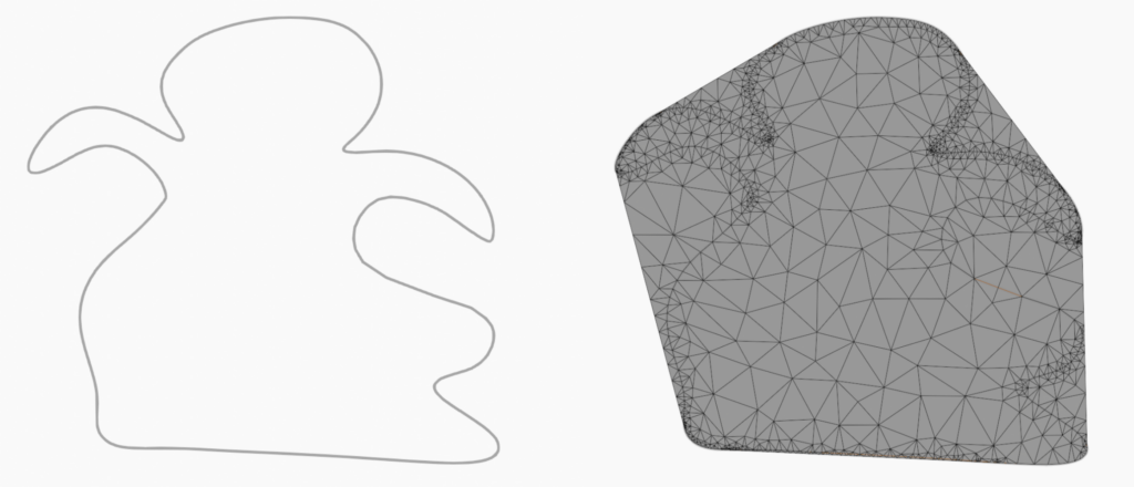
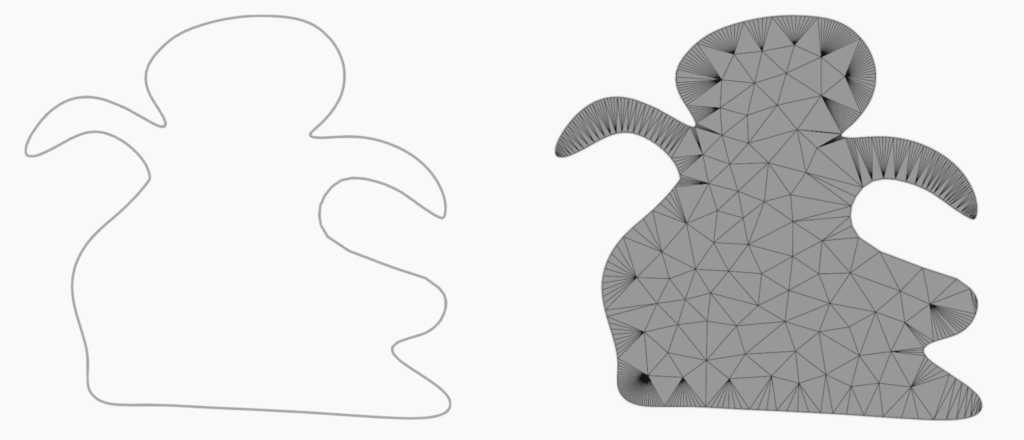
The second parameter allows to maintain the angles of the triangles above 20 degrees. Without it, we may obtain elongated triangles like that :
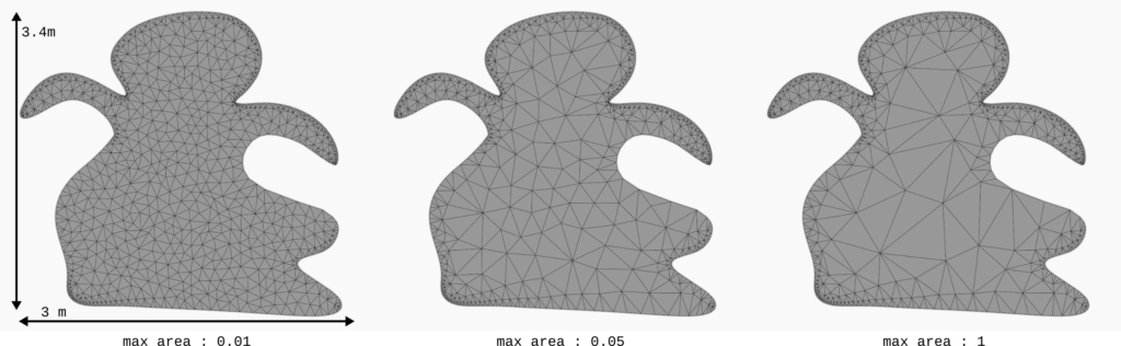
Lastly, we define a maximal surface area with the parameter -a. Here we choose 0.05 arbitrarily, but this parameter can be changed depending on the dimension of the grease pencil object or the scene.
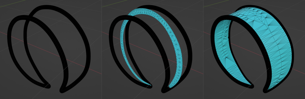
Lifting the mesh in 3D
We now have a mesh with 2D vertices, in the local frame we computed before. We can compute the world space coordinates of these vertices by using the reverse equation. The same mesh is now expressed with 3D coordinates in the plane fitting at best the stroke. If the stroke were to be planar, then our job is done, because the mesh should fit the boundaries and have the regular topology we aim at. Otherwise, we need an extra step, so that the boundary vertices of the mesh fit the stroke while keeping good mesh quality. More specifically, we would like to keep the surface smooth from discontinuities.
Minimal surfaces
Note that there are many ways to compute a smooth mesh matching the 3D boundaries. We need a criterion to lead our computation. Here, we use what’s called Laplacian minimization, which is an optimization process to minimize the mean curvature of a surface. The resulting mesh represents an approximate minimal surface.
To get a more visual idea of what’s a minimal surface, imagine the grease pencil strokes to be wires that you would dip into soapy water. The bubble-like membrane envelope around the wires represents a minimal surface. See for example this.
Implementation
Technical details of the method can be found in [Botsch and Sorkine 07]. Here is an attempt to sum it up, with as few obscure math equation as possible.
We have as input a 3D planar triangulation, meaning a set of n vertices { vi=(xi, yi, zi) }i∈{0..n-1}, along with triangular faces. We want to modify this mesh so that it fits the grease pencil stroke while keeping a minimal mean curvature. We formulate this issue as a least square minimization problem, which means that we pose a set of unknown x and a set of linear constraints expressed as matrices A and b and solve the system Ax=b. Here our unknown values are a set of n 3D displacements di=(dxi,dyi,dzi) to apply to each vertex of the mesh to get our resulting surface.
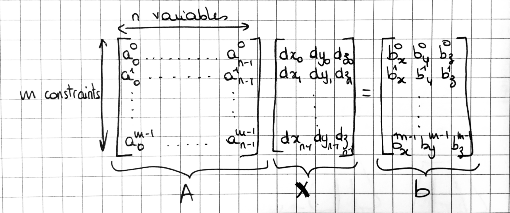
The matrices A and b define a set of constraints of the form : a0k*d0 + ... an-1k*dn-1 = bk .
Such a system can be solved using the numpy least square resolution function linalg.lstsq which returns the values of x that satisfy at best the equality Ax = b. In our case we can compute the resulting mesh by translating each vertex of the triangulation by the displacement di obtained.
Note that the equality Ax = b may not be achievable, because some constraints might be in conflict. The least square method returns the values that minimizes ∑k|| ∑i aik di -bk ||2.
The Laplacian minimization is thus expressed through the values of matrices A and b. The idea is to minimize the mean curvature of the surface at each vertex of the mesh. The mean curvature is approximated by the discretization of the Laplace-Beltrami operator, which is based on the Voronoi area of the vertices (the area of a close neighborhood of each vertex in the mesh).
The result is a matrix-based set of constraints of the form :
(-ks Ls + kb Ls M-1 Ls) x = 0,
where :
– ks, kb are the stretch and blend weights (both set to 0.5 in our implementation),
– M is a diagonal matrix containing the Voronoi area of each vertex,
– Ls is a matrix of coefficients {ωij} for i≠j and {-∑ k≠i ωki} on the diagonal,
– and ωij = 0.5*( cotan αij + cotan βij ) if (i, j) are adjacent vertices in the mesh, where ( αij, βij ) are the opposite angles to edge (i,j), and ωij = 0 otherwise.
For more details, please refer to the paper.
This provides us a good basis of a least square system that minimizes the mean curvature of a mesh, where A = (-ks Ls + kb Ls M-1 Ls), and b = 0. If we solve it as is, we obtain x=0, meaning leaving the vertices where they are. Indeed, the triangulation is initially planar, and thus its mean curvature is already minimal, it equals 0 everywhere. We need the boundary constraint to counterbalance the Laplacian minimization, and to enforce the vertices of the boundary to move away from the plane that contains the triangulation.
There are two ways to add the boundary constraint into the system :
1. Soft constraint.
We add some lines to the matrices A and b to account for additional constraints of the form : di = bi – vi , for each vertex i that belongs in the boundary of the stroke, where vi is the coordinates of the vertex in the planar triangulation, and bi the coordinates of the corresponding vertex in the boundary.
2. Hard constraint.
Alternatively, we can consider that vertices which belong in the boundary are not unknown on the system but fixed values. In this case, there is no need to add lines into the matrices, but rearrange the columns so that all coefficients corresponding to boundary vertices are moved to the right part of the equation. The matrix A thus has less columns, because there are less unknown variables.
We implemented both methods, and did not notice difference in performance in the examples we had. In theory, the second option should be best because it guarantees the boundary to be perfectly fitted, and reduces the size of the system.
Results
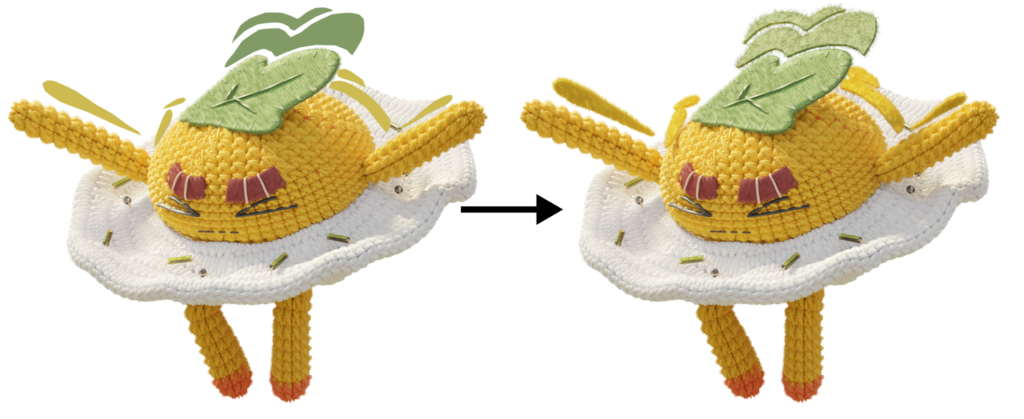
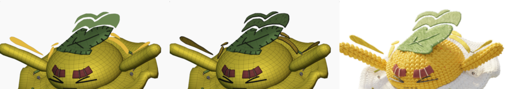
The results satisfy our needs : for most curves, the mesh is regular, and the boundary is always fitted. With a few modifiers, you can add thickness, and some bevel to result, and obtain 3D elements to be integrated to 3D animations, like these.
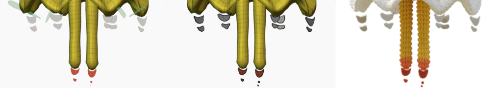
Limitations occur mainly when the projection of the input curve on the fitted plane self-overlaps. In this case, the mesh looses the topology qualities it had gained from the 2D triangulation, like in the example above.
Our algorithm also currently does not deal with holes. On the performance level, the most expensive part of the algorithm is the Laplacian optimization. Thus, it is important to only perform it if the input curve is indeed not planar.
How to get it ?
The triangulation implementation is free and available on GitLab : https://gitlab.com/lfs.coop/blender/gp-triangulation.
Note that the code to do the triangulation + laplacian optimization is (almost) contained in the laplacian.py file, and in the laplacian_triangulation function (some functions from the utils.py file are needed to make it work).
References
[Stanko et al. 16] Stanko, T., Hahmann, S., Bonneau, G. P., & Saguin-Sprynski, N. (2016). Surfacing curve networks with normal control. Computers & Graphics, 60, 1-8.
[Shewchuk 96] Shewchuk, J. R. (1996, May). Triangle: Engineering a 2D quality mesh generator and Delaunay triangulator. In Workshop on Applied Computational Geometry (pp. 203-222). Springer, Berlin, Heidelberg.
[Botsch and Sorkine 07] Botsch, M., & Sorkine, O. (2007). On linear variational surface deformation methods. IEEE transactions on visualization and computer graphics, 14(1), 213-230.
3 Comments
Henri Hebeisen
Amazing work, congratulations ! 🙂
Lewis
Hey, this is a great addon! I’m experiencing crashes whenever I convert a Grease Pencil object traced from an image – sometimes it’ll work properly when I duplicate the object or alter its geometry. Is it something to do with how Blender stores the object’s id? I noticed I also can’t copy the traced Grease Pencil object to other instances of Blender. Any help would be appreciated. Thanks so much!
Amélie
Hi,
Thanks for your comment, and sorry for the large delay, we don’t check this comment section very often, as you can see.
If you still experiment issues on this topic, I would appreciate if you could report it as an issue on gitlab : https://gitlab.com/lfs.coop/blender/gp-triangulation/-/issues .
It’s easier for us to look into it 🙂