In our article on the making of Antarctica, we used Open Street Map (OSM) to obtain the coordinates of points with which we can create a closed line, representing the coast boundaries of the Antarctic continent. In this article, we will explain how we send a request to the Overpass turbo server to get filtered data, then we show how we have manipulated the data in Blender to get a Antarctic Polar Stereographic projection (in the WGS84 coordinate system).
Open Street Map and Overpass turbo
OSM is a project to create a world map constructed with free geographic data and people contributions, all under free/libre licence. For exemple, it is widely used in popular services which need a locator map.
Although an addon exists for Blender which does some of the things described in this article (BlenderGIS), it proved quite hard to install on our environment, and there were some limitations which we couldn’t overcome, such as the limited extent to which one may make overpass queries.
Overpass turbo is a interactive web based data filtering tool for OSM which can run Overpass API queries and shows the results on an interactive map. This project is maintained by Martin Raifer (GitHub).
Data mining
To obtain the coast boundaries of the Antarctica continent in Overpass turbo, we used the following query:
[code]
[out:json];
way["natural"="coastline"](-90,-180,-60,180);
(._;>);
out;
.1;
[/code]
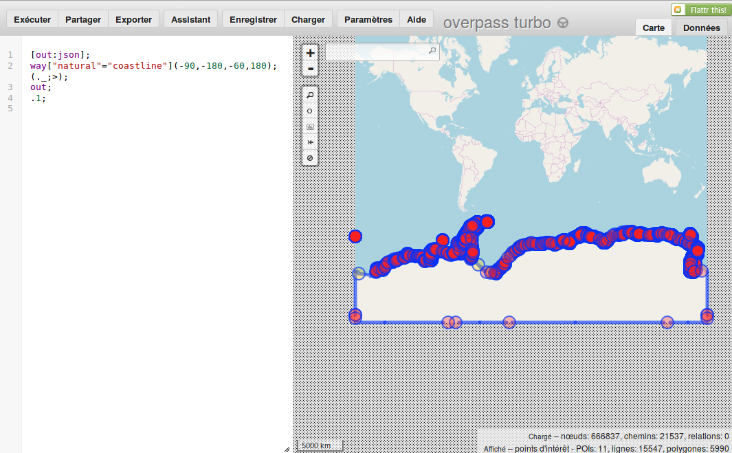
Figure 1. Overpass Turbo.
[out:json]; allows getting the raw data in the JSON export format.
The second line gets all the coast boundaries under the latitude -60°, where there is only the Antartica continent.
Then we export the data with the export button, then the raw data format to get the JSON file we want.
Data manipulation
To parse and import the JSON data into Blender, we wrote this python script, which create a curve object (Figure 1):
[code lang=”python”]
”’Parse OSM DATA and create curve
”’
import bpy
import json
from math import pi
with open(‘/path/to/interpreter.json’, ‘r’) as f:
data = f.read()
json_data = json.loads(data)
nodes = {el["id"]:el for el in json_data["elements"]}
ways = (el for el in json_data["elements"] if el["type"] == "way")
curve = bpy.data.curves.new("Coast", ‘CURVE’)
ob = bpy.data.objects.new("Coast", curve)
for way in ways:
spline = curve.splines.new(‘POLY’)
spline.points.add(len(way["nodes"])-1)
for i, wnode in enumerate(way["nodes"]):
node = nodes[wnode]
point = spline.points[i]
# web mercator EPSG:3857
point.co[1] = node["lat"]
point.co[0] = node["lon"]
bpy.context.scene.objects.link(ob)
[/code]

Figure 2. Curve object (orange) created from the imported data. Note the bottom line, which we’ll get rid of later on. The black and white plane is that mentioned in a previous article, for comparison.
We now convert the curve to a mesh to get a polygonal line.
The data from OSM is in the web mercator EPSG:3857 projection in the standard WGS84 spatial reference. It is well suited to represent the whole globe but the poles appear very distorted. So we wrote a python script leveraging the pyproj module to reproject our data in a polar projection (Antarctic Polar Stereographic projection), centered on the Antarctic continent, with an acceptable deformation which made the continent identifiable.
[code lang=”python”]
”’Reproject polyline to Antarctic Polar Stereographic (WGS84)
”’
import bpy
import pyproj
polar=pyproj.Proj("+init=EPSG:3031") # WGS 84 / Antarctic Polar Stereographic
latlong_ob = bpy.context.object
verts = []
for v in latlong_ob.data.vertices:
x, y = polar(v.co[0], v.co[1])
verts.append((x/10**7, y/10**7, 0.0))
faces = [p.vertices for p in latlong_ob.data.polygons]
edges = []
edges = [e.vertices for e in latlong_ob.data.edges]
polar_mesh = bpy.data.meshes.new(‘Polar’)
polar_mesh.from_pydata(verts, edges, faces)
polar_ob = bpy.data.objects.new(‘Polar’, polar_mesh)
bpy.context.scene.objects.link(polar_ob)
bpy.ops.object.join_uvs()
bpy.ops.object.make_links_data(type=’MATERIAL’)
[/code]
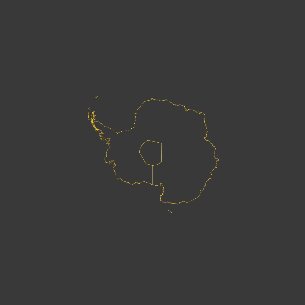
Figure 3. Reprojected mesh with remaining pole lines.
The mesh now has its final shape, but it needs to be cleaned up by deleting all the points at the center, which formed the border of the square in the previous projection. We can now fill in the faces to get a usable mesh (Figure 3).
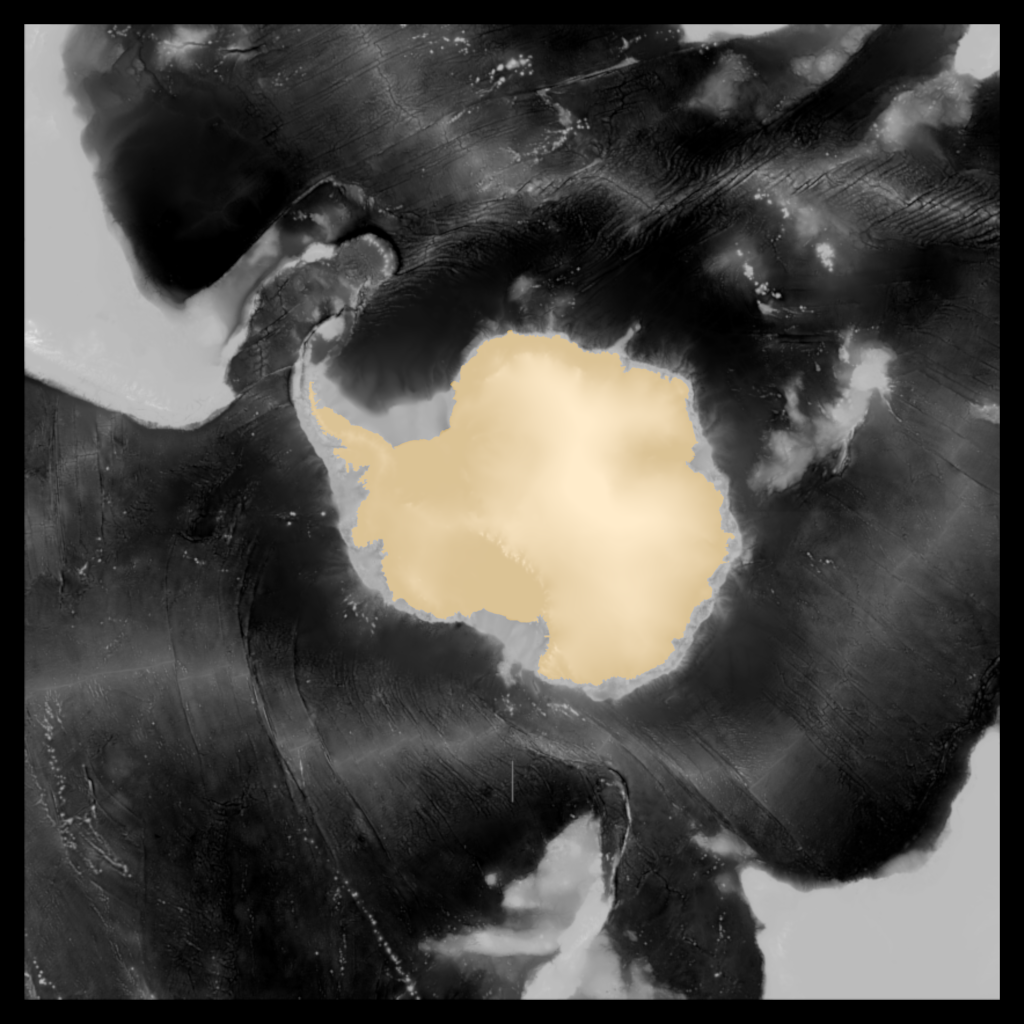
Figure 4. Final mesh, with filled faces. It matches the QGIS projection very well.
And that is how we got the result we needed, the Antarctica continent with the least possible deformation.
Acknowledgements
The data used are credited to:
- OpenStreetMap