Antarctica is a documentary directed by Jérôme Bouvier and Marianne Cramer co-produced by Arte France, Paprika Films, Wild-Touch Production, Andromède Océanologie. It depicts the expedition led by Luc Jacquet to show and raise interest in the effects of climate change in the polar regions.
We produced animated sequences to illustrate the two films with cartographic images, to show natural phenomenons about the oceanic current, circumpolar current, ice melting, etc. We have also made “overlay graphics ?” to show how the fauna is adapted to the harsh climate.
In this article, we show two experimental processes using scientific data to make our cartographic animated sequences, with art direction by Eric Serre.
1) 3D Earth reconstruction
For this project, we reconstructed the entire earth and a tile map centred on the Antarctica. We needed high fidelity of the coast delimitation and of the altimetry and bathymetry (altitudes of continents and ocean floors).
NASA provide the land topography (Figure 1) of the Earth’s surface with the elevation data collected by space-based radars.
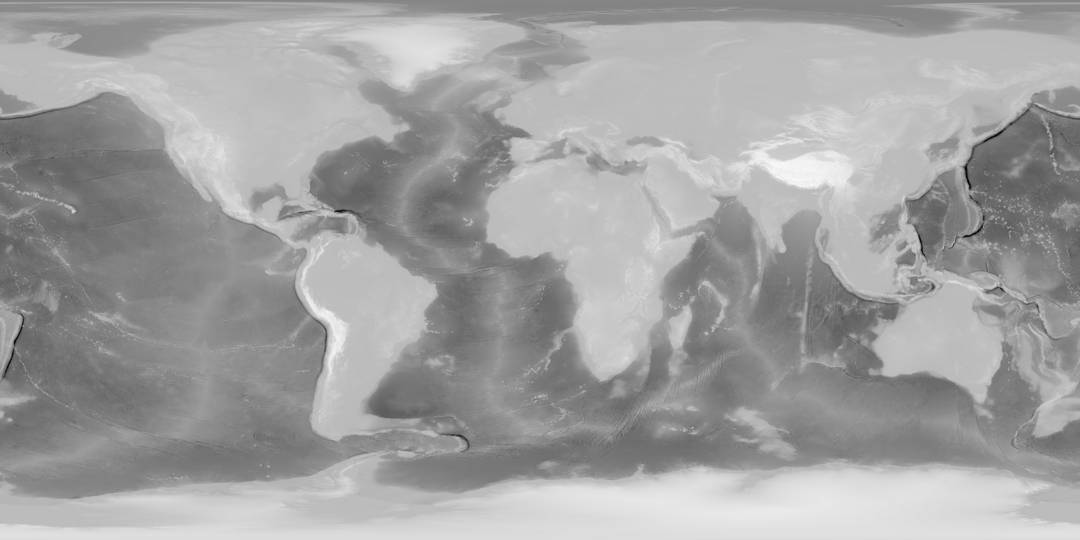
Figure 1. Land topography of the Earth surface. Modified imagery by Jesse Allen, NASA’s Earth Observatory, using data from the General Bathymetric Chart of the Oceans (GEBCO) produced by the British Oceanographic Data Centre.
The projection used is the standard WGS84, an equirectangular type. It is well suited to represent the whole globe but not for just a smaller part. This is even worse for the poles, which appear very distorted. With the help of GIS (Geographic Information Systems) software QGIS, we were able to reproject the map to a polar projection (Antarctic Polar Stereographic), centred on the Antarctic continent, with an acceptable deformation which made the continent identifiable (Figure 2).
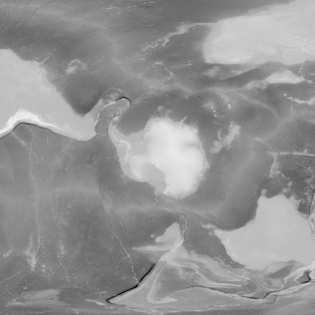
Figure 2. Polar projection centred on the Antarctic continent.
These two topography maps, also called height maps, can be used to reconstruct the Earth using the displacement mapping technique, where the geometric position of points on a surface are displaced along the height. The height maps are usually greyscale images where black represent the lowest elevation, and white the highest elevation.
To determine the water height, we can compare the height maps with the open data given by Open Street Map. With a request to the server, we obtain the coordinates of points with which we can create a closed line, representing the coast boundaries of the Antarctic continent (Figure 3).
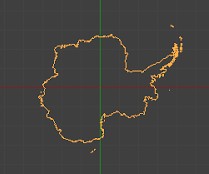
Figure 3. Coast boundaries obtained from the Open Street Map data.
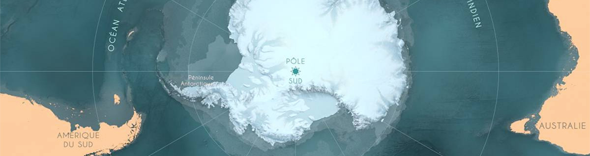
With all these data collected, we were able to reconstruct the Earth and a cropped area centred on the Antarctic continent which is depicted on Figure 4.
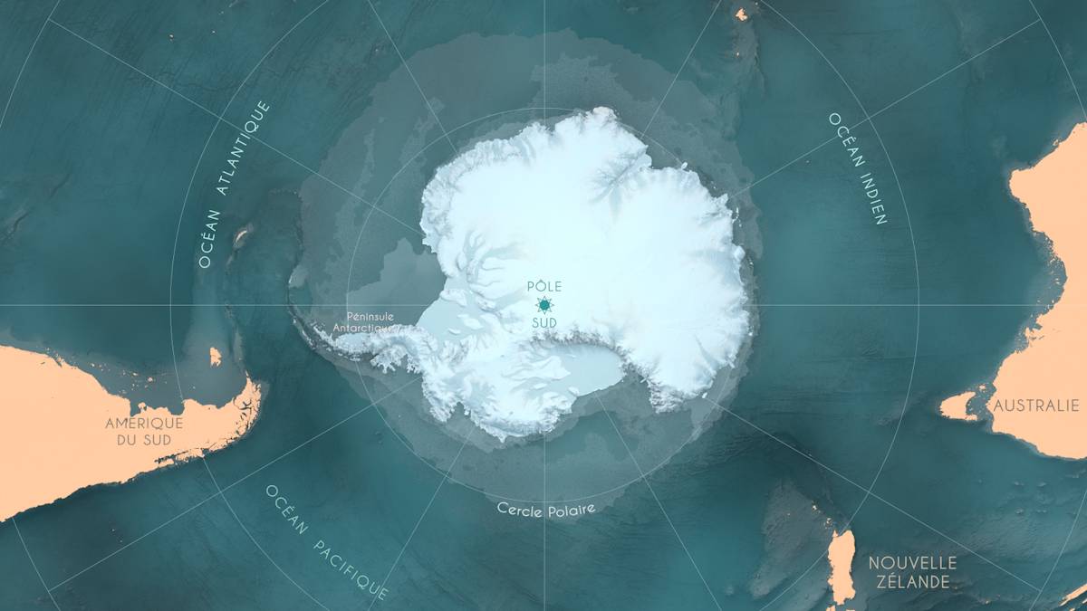
Figure 4. Composited render of the Antarctic continent tile map.
2) Ice melting flow
We had to create an animated sequence representing the ice melting flow of the Antarctic glacier. To obtain enough fidelity on the glacier region and the ice melting flow, we used data from the National Snow and Ice Data Center in the United States.
The data provided are two maps with a spatial resolution of 450 meters per pixel on a map of 12445×12445 points, or a spatial resolution of 900 meters on a map of 6223×6223 points. It represents the speed vector of the water flow in one year, that is to say the direction of propagation and the value distance of the movement.
To compute the data, we used Processing, a graphical programming environment, to create a simple program to parse the data and a particle system which consists of a simple launch of particles, moving following the direction and speed defined by the vector at their position, at each frame. The resulting images are used as an animated mask to create the water flow in the final result. In Figure 5, we depict the three types of passes we used, a zoom and the compositing of only the 3 passes. Figure 5.a is the glacier pass obtained with the first frame of the simulation with one particle at each point of the map. Figure 5.bc are the ice melting flow passes, obtained with a particle density 5 times lower than the vector map resolution. Figure 5.c has a threshold to limit to the highest flows and permit to have higher dynamics on the value. The 3 passes are composited as shown in Figure 5.e, and we obtain the final compositing result on Figure 5.f.
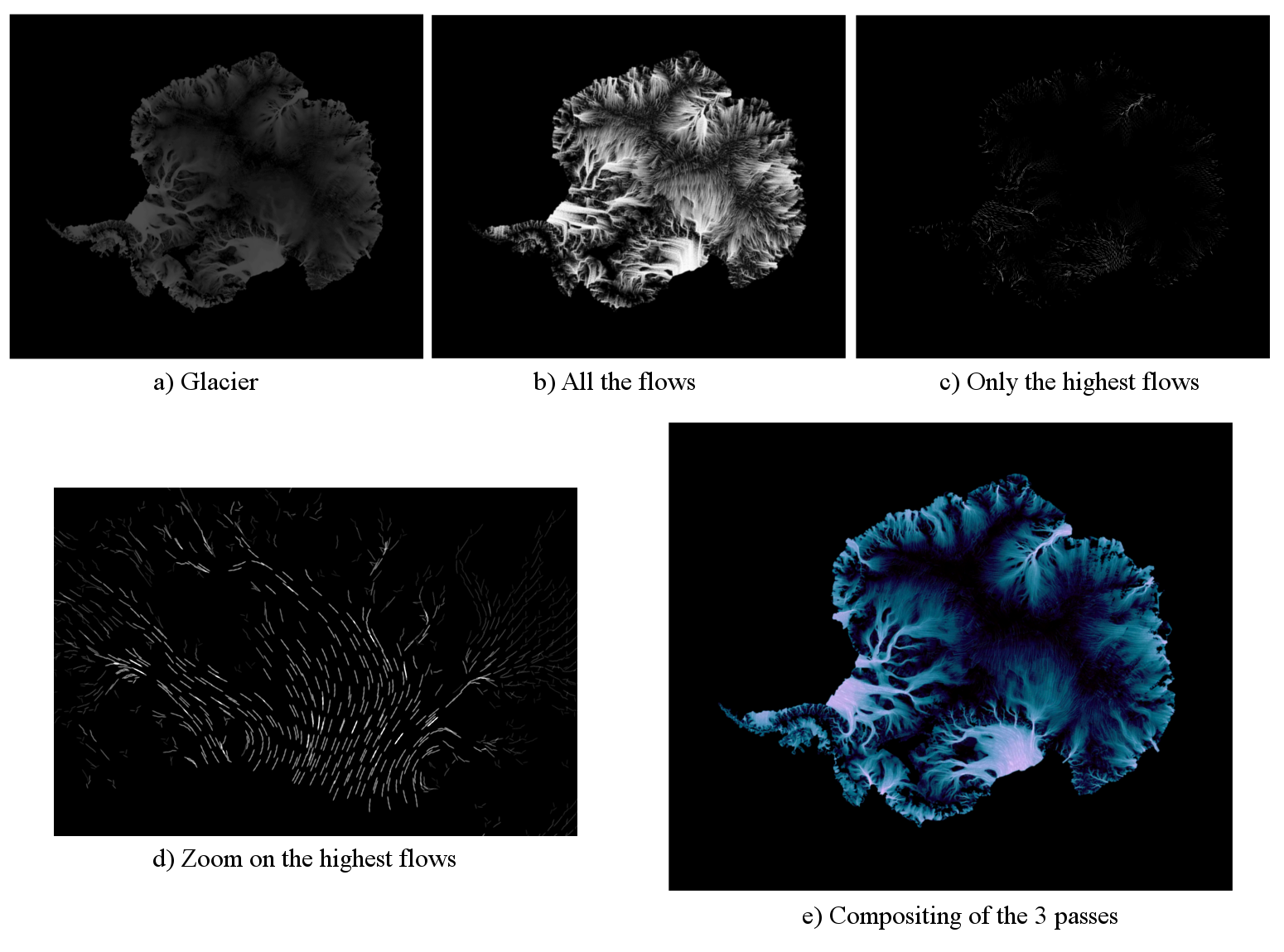
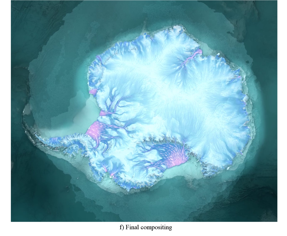
Figure 5. Process to add the ice melting flow to the final compositing
Acknowledgements
The data used are credited to :
- Imagery by Jesse Allen, NASA's Earth Observatory, using data from the General Bathymetric Chart of the Oceans (GEBCO) produced by the British Oceanographic Data Centre.
- Rignot, E., J. Mouginot, and B. Scheuchl. 2011. MEaSUREs InSAR-Based Antarctica Ice Velocity Map [indicate subset used]. Boulder, Colorado USA: NASA DAAC at the National Snow and Ice Data Center. doi:10.5067/MEASURES/CRYOSPHERE/nsidc-0484.001

The work presented here is produced with free/libre and open source software: GNU/Linux, Blender, Natron, Processing, Open Street Map, QGIS.
3 Comments
Antoine Blais
Bonjour Kévin,
Ton article est vraiment sympa 🙂 Je l’ai fait passer au labo.
J’avais zappé qu’il y avait un atelier prévu samedi 3 février …
Sais-tu quand est programmé le prochain ?
Antoine
Thomas
C’est magnifique d’avoir utilisé des outils open-source de cartographie et Blender pour rendre quelque chose de visuellement impactant avec un peu de rigueur scientifique. Je suis un peu interrogatif de voir de si beaux projets ne pas avoir l’écho qu’ils devraient avoir. J’adore Blender. J’adore la science et l’océanographie. J’aime beaucoup ce que vous faites en communication scientifique et technique.